N-Puzzle Algorithms
Efficient N-Puzzle Algorithms
Table of Contents
- Efficient N-Puzzle Algorithms
- Breadth First Search
- Heuristics
- Optimal Search Algorithms
- Fast Search Modificiations (Any Path)
What is an N puzzle?
The N puzzle, also referred to as the sliding tile puzzle, is a simple game. You are provided a square board of tiles numbered 1-N with one blank tile.
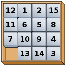
The goal is to slide tiles, exchanging them with the blank square until they are in ascending numerical order. The blank tile will either be in the first or last square, depending on the goal. Common games of the N Puzzle are the 8-puzzle, 15-puzzle, 24-puzzle, and 35-puzzle. These games are of interest for search and pathfinding algorithms due to the size of the search space that renders standard algorithms ineffective.
The search space for the 8 puzzle is relatively small at only 362880 possible states. This makes it possible to search the entire space in a short time. However, once you move to the 15 puzzle, it jumps to 1,307,674,368,000 possible states. As you can imagine, the 24 and 35 puzzles are much too large to search in a finite amount of time.
Breadth First Search
Heuristics
For a heuristic to work for this problem, it must be admissable. An admissable heuristic means that it must provide a lower bound on the number of moves to reach the goal state. This means that it must take at least the expected number of moves to reach the goal state and not any more. If it were to overestimate the number of moves, it can miss the shortest path.
There are instances where you could use an inadmissable heuristic to solve the puzzle, but for my purposes, I will be searching for an optimal solution.
Misplaced Tiles
The misplaced tiles heuristic is a simple one, and simple to compute. It is simply the total number of tiles that are out of place. This is admissable because it must take at least one move to get a misplaced tile into its correct spot.
Manhattan Distance
More complex than the previous one, but much more effecive, is manhattan distance. The manhattan distance is the sum of the differences between the x and y coordinates between the position of each tile compared to its goal position. g(x) is the goal position of the x tile and s(x) is the current position of the x tile.
\[M = \sum_{i=1}^N |g(i)_x - s(i)_x| + |g(i)_y - s(i)_y\]Linear Conflict
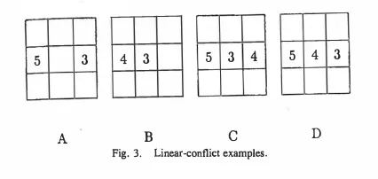
An additional heuristic, further complicated, is the linear conflict heuristic. This can actually be combined with the manhattan distance heuristic. Linear conflict is the number of pairs of tiles that are in their correct row or column, but are reversed relative to their goal positions. This can be added to the manhattan distance heuristic for an improved heuristic function.
Pattern Databases
An alternative heuristic, particularly useful for solving the larger 15, 24, and 35 puzzles, are pattern databases. Pattern databases have been the focus of significant research, particularly as they were being first discovered in the early 2000s. The nomenclature has evolved from the beginnings, so you will see them called different things depending on the paper you look at. The common way to refer to them now are:
- Non-additive
- Additive
- Statically partitioned
- Dynamically partitioned
We will focus on statically partitioned additive pattern database heuristics (what a mouthful), but you can read about the rest in the source paper. Pattern databases rely on storing the exact number of moves it takes for a subset of tiles (static partitioning) to reach their goal postiions from any other position on the board. You are able to add together the number of moves from multiple databases so long as they are disjoint, i.e. a tile cannot be in multiple pattern databases. All tiles must appear in a database for it to be admissable. Notably, the blank space is ignored when looking up a state in the database.
Computing the Database
Computing the database is fairly straightforward. You run a reverse breadth first search on the goal state, but with every other tile not in the pattern set as -1. You can get neighboring states in one of two ways:
- Find every open square adjacent to a pattern tile. Switch positions with that tile and add 1 to the path cost.
- Start a search from the goal state with every open position adjacent to a pattern tile. Place a blank tile there and run breadth first search. Only increase the path cost if the blank tile switches with a pattern tile.
For any state already in the database, store only the minumum path cost.
For the 8-puzzle, you could easily store the entire board as a pattern (resulting in a heuristic lookup table). However, for larger boards, specific partitions may work better (but use more memory).
For the 15-puzzle the original paper tries three patterns:
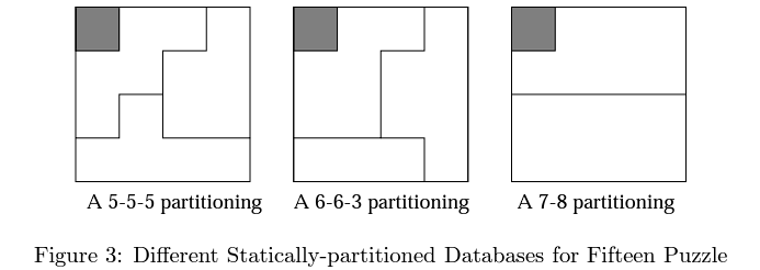
They found that the 7-8 pattern was the fastest, thought it was also the largest. I recommend exploring that paper if you want to tackle larger puzzles.
Indexing the Database
There are many ways you could encode the state to store it in the database, but I choose a fairly simple approach. I encode it by putting the x and y coordinates of each pattern tile (in numerical order) into a string. This is the key for the database. Again, note that the blank tile position is not considered.
Optimal Search Algorithms
I will discuss some of the heuristic search algorithms one might use to find an optimal path for solving the N puzzle.
A*
A* search is the quintessential heuristic search algorithm. It works well for the 8 puzzle and can be applide to larger puzzles, but memory constraints start to become a concern due to needing to store previously seen states (closed set). For pseudo-code for A, see link. For a recent and interesting explanation for how A works (a great watch even if you already know A*, it’s a very interesting exploration) is this YouTube video.
It is straightforward to implement, you just add in your heuristic function. Using a priority queue for the open set, the priority of a state is f(x) = g(x) + h(x), i.e. the priority of a state is the sum of its path cost and heuristic value. One additional difference between BFS and A* search is that the closed set is not immutable. When checking child states, if you are searching for an optimal path, you must check if the path cost of the child state is less than the path cost of the state in the closed set. See pseudocode below for an example of this:
for child_state in expand(state):
  if child_state not in closed_set or child_state.path_cost < closed_set[child_state].path_cost:
    closed_set[child.state] = child  # update closed set with shortest path seen for the given state
In Python, this code could be simplified by using a defaultdict for the closed set:
from collections import defaultdict
closed_set = defaultdict(yield float('inf)) # default value is positive infinity
...
for child_state in expand(state):
  if child_state.path_cost < closed_set[child_state]: # if not found, defaultdict will return the default value of positive infinity
    closed_set[child_state] = child_state.path_cost  # update closed set with shortest path seen for the given state
...
IDA*
For the larger puzzles, memory constraints become a significant problem. If you are using pattern databases, you already use may already be using a considerable amount of memory.
In this case, you will likely want to use Iterative Deepning A* Search (IDA*). This gets rid of needing to store a set of previously seen states by only searching a given state up to a certain depth before returning, checking all other available states. If the goal was not found, then the depth bound is increased to the next lowest priority seen during exploration (path cost + heuristic).
Pseudocode for IDA* can be found on Wikipedia
Fast Search Modificiations (Any Path)
To search for any path to the goal quickly, but not necessarily the shortest path, only a small modification needs to be made to the A* algorithm.
- Use a set for the closed set.
- You do not need to worry about the shortest path seen, so ignore all states if you have seen them before.
- Prioritize new states only by their heuristic value.
This is known as Greedy Breadth First Search. While not technically A* any longer, you can implement it via Weighted A* search, where you multiply the g(x) value from before by $\lambda_g$. When you want an optimal path, $\lambda_g = 1$ and when you want speed $\lambda_g = 0$.
Expanding child/neighbor states will look as follows:
for child_state in expand(state):
  if child_state not in closed_set:
    closed_set.add(child_state)
    open_set.add(child_state, priority=get_priority(child_state, lambda_g=0))